A chargeability anomaly that looks like a porphyry target and turns out to be graphitic shale is a wasted drill hole, a budget hit, and a credibility problem in front of your board. Reading an IP pseudosection correctly before the rig mobilizes is one of the highest-leverage skills in a pre-drill exploration workflow, and it is not something most geophysics textbooks treat with the practical directness the job demands.
This article walks through how to read a dipole-dipole IP pseudosection in a field context: what the geometry of the plot actually represents, how to distinguish a sulfide target from a conductive artifact, how to estimate depth from apparent resistivity patterns, and how to use chargeability and resistivity together to make defensible pre-drill decisions. For a full overview of survey design, array selection, and data acquisition standards, see Rangefront’s induced polarization survey services page.
What a Pseudosection Actually Shows (And What It Doesn’t)
A pseudosection is a plot of apparent resistivity or chargeability values arranged by electrode position on the horizontal axis and n-spacing on the vertical axis, where each datum is plotted at the midpoint of the transmitter-receiver pair and at a pseudo-depth defined by a geometric convention.
That pseudo-depth does not correspond to a real physical depth. A datum plotted at n=4 spacing on a dipole-dipole array is not coming from four times the electrode spacing in depth. The actual depth of investigation for that datum is shallower than the plot implies, typically in the range of 15 to 25 percent of the total transmitter-receiver separation depending on subsurface resistivity contrasts. Treating the vertical axis as a true depth scale is the most common misreading in field interpretation.
What the pseudosection does show accurately is the lateral position and relative strength of anomalies. If you see a strong chargeability high centered at station 400 E on n=3 through n=6 spacings, there is a real chargeable body near that location. The plot’s geometry tells you where to look; inversion tells you how deep and how large.
Anatomy of a Dipole-Dipole Pseudosection
A standard dipole-dipole pseudosection uses equal transmitter and receiver dipole lengths (a-spacing) and varies the separation between them in integer multiples (n = 1, 2, 3, 4, 5, 6). The resulting data points form an inverted-V shape in the plot space, with the shallow measurements (n=1, 2) across the top and the deepest apparent measurements (n=5, 6) at the bottom.
This geometry creates a characteristic visual signature for any discrete conductive or chargeable body: the anomaly appears as a downward-pointing cusp or inverted-V pattern that narrows with depth. A spherical body at depth will produce a symmetrical cusp centered above it. An elongated body, like a steeply dipping sulfide zone, will produce an asymmetric or offset cusp depending on dip direction. Recognizing these shapes is the foundation of field-level pseudosection reading.
At the edges of the pseudosection, which are the first and last few stations, the geometry produces artifacts. With fewer electrode positions contributing to the deepest data points, the apparent values at the corners are unreliable. Flag those corner datums and do not interpret them as anomalies.
Reading Chargeability: Sulfides vs. Artifacts
Chargeability measures the degree to which a material stores and slowly releases electrical charge after current is switched off. Sulfide minerals such as pyrite, chalcopyrite, sphalerite, molybdenite, and galena are strongly chargeable. So are graphitic carbon phases and, to a lesser degree, clay minerals under certain pore-fluid conditions.
A sulfide chargeability anomaly in a porphyry or epithermal system typically presents as a broad, high-amplitude zone (greater than 15 to 20 mV/V in many Western US and Canadian settings) that correlates spatially with a resistivity low, indicating a disseminated sulfide-bearing zone with moderate conductivity from both metallic conduction and pore fluids. The anomaly has smooth lateral margins and deepens progressively from the surface trace of mineralization inward.
Graphitic shale produces a chargeability response that is often higher amplitude and more laterally continuous than sulfide mineralization. The key distinction is the resistivity signature. Graphite is an excellent conductor; a graphitic horizon will produce a strong chargeability high sitting directly on top of a sharp, low-resistivity layer that is both laterally consistent and geologically mappable as a stratigraphy unit. If your chargeability anomaly tracks a resistivity contour that runs parallel to regional strike and does not show any cusp geometry, treat it as a probable graphitic horizon and verify with geology before drilling.
Clay alteration produces a weak, diffuse chargeability response rarely exceeding 5 to 8 mV/V in most field conditions. It is not a drilling target on its own, but a clay chargeability halo that surrounds a stronger sulfide anomaly is geologically coherent and supportive of a mineralized system interpretation.
Reading Resistivity: What Low and High Values Mean in Context
Resistivity in a pseudosection is interpreted relative to the regional background. There is no universal value that means “mineralized.” A 100 ohm-m body is highly resistive in a graphite-bearing metasedimentary terrain and unremarkable in a granite-hosted porphyry setting.
That said, several resistivity patterns recur across Western US and Canadian mineral systems.
In porphyry Cu-Au-Mo systems, the potassic core typically presents as a moderate-to-high resistivity zone reflecting fresh, K-silicate altered rock with disseminated sulfides. The phyllic/argillic shell surrounding it is often lower resistivity due to clay alteration and increased sulfide content. The IP target is the transition zone between the potassic core and the phyllic overprint, where chargeability is highest and resistivity is transitional.
In Carlin-type systems in Nevada, resistivity contrasts often track structural controls: high-angle faults and decalcified silty carbonate units produce resistivity lows, while silicified cap rocks produce highs. IP is less diagnostic for gold in Carlin settings than for sulfide-associated gold in other deposit types, but resistivity patterns can still define structural corridors worth drilling.
In epithermal Au-Ag systems, high-resistivity zones at shallow depths often correspond to silicified structures or vein corridors. If those high-resistivity zones have even moderate chargeability values (5 to 12 mV/V), they warrant further investigation. Low-sulfidation epithermal systems may show modest IP responses overall; intermediate and high-sulfidation systems tend to produce stronger chargeability due to higher total sulfide content.
The Coincidence Test: Why You Need Both Plots on the Same Screen
The single most important interpretive habit for pseudosection work is running the chargeability and resistivity plots together on the same horizontal scale before drawing any conclusions. A chargeability anomaly without a corresponding resistivity feature is ambiguous. A resistivity anomaly without a chargeability response is probably structural or lithologic, not a sulfide target.
The targets worth drilling show both: a chargeability high that is spatially coincident with either a resistivity low (disseminated sulfides with conductive matrix) or, in silica-dominant systems, a resistivity high. The spatial offset between the chargeability peak and the resistivity feature is itself geologically interpretable. If the resistivity low is 50 to 100 meters up-dip of the chargeability high, that pattern is consistent with a steeply dipping sulfide body where the conductive portion is shallower and the chargeable zone extends at depth.
This coincidence test is not infallible; some valid targets show modest resistivity contrast. But it is the fastest way to separate signal from noise in a multi-line pseudosection dataset, and it is the check that should happen before any line is promoted to the drill-target list.
Depth Estimation from Pseudosection Geometry
Getting a useful depth estimate from a pseudosection without inversion requires a working knowledge of the depth sensitivity rules for dipole-dipole geometry. The commonly cited approximation is that the effective depth of investigation for a dipole-dipole array is roughly 0.17 times the total transmitter-receiver separation (na), where n is the spacing multiplier and a is the electrode spacing.
For a 100-meter a-spacing array at n=4, the effective depth of investigation is approximately 0.17 × 400 m = 68 meters. For n=6, it is approximately 102 meters. These are conservative estimates; the actual depth depends on the resistivity structure, and in conductive cover, investigation depth decreases.
In practice, the top of a target anomaly in the pseudosection plot approximates its shallowest edge. If a chargeability cusp first appears at n=2 and reaches maximum amplitude at n=4, the top of the body is likely within the depth range corresponding to n=2 to n=3 spacing. That bracketing gives you a starting depth for drill planning, not a confirmed target depth. Confirmed depth requires inversion.
When depth matters for collar design and budget planning, two-dimensional inversion using software such as Res2DInv or ZondRes2D is worth the processing time. The pseudosection gives you the target location; inversion gives you the geometry.
From 2D Pseudosection to 3D Understanding
A single survey line gives you a 2D slice. Most ore bodies are three-dimensional, and interpreting a drilling program from a single line pseudosection is a known source of mis-targeting. If a chargeability anomaly appears on line 1000 N but not on line 800 N or 1200 N, you are either at the lateral margin of the target or the anomaly is a line-specific artifact from a shallow, linear conductive feature parallel to the survey line.
Multi-line pseudosection programs, where lines are run at regular intervals (typically 50 to 200 meters depending on target size), allow you to fence the anomaly laterally and begin building a mental 3D model before formal inversion. When you plot the peak chargeability value from each line at the same n-spacing on a map view, you get an approximate plan-view footprint of the target. That map is one of the most useful pre-drill documents you can have.
Formal 3D inversion using the UBC-GIF suite or VOXI Earth Modelling takes this further, converting multi-line pseudosection data into a volumetric chargeability and resistivity model that can be co-rendered with geology and drill collar plans. For programs where NI 43-101 technical report documentation is required, that 3D model is also the format needed to support [technical reporting services](https://rangefront.com/technical-reporting/) requirements around target definition and exploration rationale.
For programs where budget allows, merging the IP 3D inversion result with gravity or magnetic inversion in an integrated 3D geological modeling workflow produces a more constrained target volume than any single method alone.
Common Misinterpretations and How to Catch Them
- Mistaking electrode coupling problems for anomalies. Poor electrode coupling, such as with dry ground, frozen active layer, rocky terrain with no soil contact, produces high-contact-resistance readings that appear as localized resistivity spikes in the pseudosection. These are almost always at single stations and single n-spacings. Real anomalies are spatially smooth. Any single-datum spike that does not repeat at adjacent spacings is a data quality issue, not a target.
- Overinterpreting endpoints. The corner data points at n=5 and n=6 at the first and last stations of a survey line have poor geometric coverage and unreliable values. Many interpreters reflexively shade these as targets because the color scale puts them in the high-chargeability range. Flag the corners and confirm any apparent anomaly there by extending the line or running a cross-line before acting on it.
- Confusing current channeling with deep mineralization. A highly conductive shallow layer, such as a saline horizon, a clay-rich regolith, or a graphitic formation, will channel current away from depth, dramatically reducing sensitivity to anything below it. In those conditions, the deep n-spacings in a dipole-dipole pseudosection are not seeing deep mineralization; they are seeing the effect of the shallow conductor. Switching to a pole-dipole or pole-pole array, which uses a remote current electrode, partly addresses this. Understanding when your array geometry is blind is as important as knowing what it can see.
- Treating high chargeability as automatically equivalent to economic mineralization. IP detects chargeable material. Economic cut-off grades require a specific sulfide species, a specific metal tenor, and a specific geometry of mineralization. A strong IP anomaly tells you there is chargeable material worth investigating, not that there is a resource. The distinction matters when communicating to project managers and investors.
Connecting Pseudosection Interpretation to Pre-Drill Decision Making
The practical output of pseudosection interpretation is a ranked target list with associated drill collar recommendations. For each ranked target, the documentation should include: the survey line and station range of the anomaly, the n-spacing range over which it is expressed, the peak chargeability value and background value, the coincident resistivity character, the estimated depth to top of anomaly, and any geologic constraints (surface sampling, mapping, prior hole data) that support or refute the IP interpretation.
That documentation is not bureaucratic overhead. It is the record of the interpretive reasoning that justified the drill decision. When a hole intersects the target, or misses it, the ability to go back and understand whether the interpretation was correct, or whether the geology was more complex than the survey could resolve, is how exploration programs improve over time.
For programs reporting under NI 43-101 technical report standards or S-K 1300 (SEC) requirements, the qualified person sign-off on exploration targets requires exactly this kind of documented interpretation chain. The pseudosection is the primary supporting figure for that documentation.
Rangefront’s geophysical survey services include both acquisition and interpretation, so the team delivering the pseudosection data is the same team that can walk through target ranking with your geological staff and help build the pre-drill documentation package.
Induced Polarization —
Technical Questions
Technical answers on pseudosection interpretation, drill targeting, mineral discrimination, depth of investigation, and NI 43-101 reporting requirements — from Rangefront's geophysical team.

ABOUT THE AUTHOR
BRIAN GOSS
President, Rangefront Mining Services
Brian Goss brings over 20 years of experience in gold and mineral exploration. He is the founder and President of Rangefront, a premier geological services and mining consulting company that caters to a large spectrum of clients in the mining and minerals exploration industries. Brian is also a director of Lithium Corp. (OTCQB: LTUM), an exploration stage company specializing in energy storage minerals and from 2014 to 2017, he fulfilled the role of President and Director of Graphite Corp. (OTCQB: GRPH), an exploration stage that specialized in the development of graphite properties. Prior to founding Rangefront, Brian worked as a staff geologist for Centerra Gold on the REN project, as well as various exploration and development projects in the Western United States and Michigan. Brian Goss holds a Bachelor of Science Degree with a major in Geology from Wayne State University in Michigan.
You may also be interested in...

Annual Claim Renewals Updated for 2026: Mining Claim Maintenance & Assessment Information
Late summer is a critical time for the mining and exploration industry. The deadline for Annual Mining Claim Renewals is September 1, and it arrives fast. Whether you’re a small-scale prospector or managing dozens of claims, it’s essential to ensure your filings,...
Combining Drone and Ground Mag Surveys: More Data, Less Time in the Field
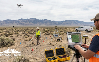
A magnetic survey is only as good as the data density behind it. Two survey platforms, flown and walked over the same ground on the same program, can double that density without doubling your budget or your schedule. That is the logic behind Rangefront's approach to...
Yukon Geophysical Surveys: Season Planning and Field Logistics
The Yukon exploration season is shorter than most project managers account for, and the margin for a poorly timed mobilization is close to zero. Between spring break-up, permafrost thaw cycles, and the onset of fall freeze, the usable field window for most ground...
Mineral Exploration in the Abitibi Greenstone Belt: Geology, Deposit Types, and What to Expect in the Field
Image Source: https://www.sciencedirect.com/science/article/abs/pii/S016913682100247X The Abitibi Greenstone Belt produced more gold than almost any other Archean terrane on Earth, and the ground is still generating discovery-stage programs across northern Ontario and...
Beyond the Borehole: How 3D Geotechnical Modeling is De-Risking Modern Mine Design
The difference between a viable project and a costly oversight lies in the "digital twin" of the subsurface. Traditional 2D cross-sections, once the industry standard, are no longer sufficient for the complexities of modern resource extraction and the stringent safety...

Starting a Geology Career in Mining and Mineral Exploration
Graduating with a geology degree opens doors, but it can be hard to know which ones to walk through first. Many new graduates want work that's hands-on, technically meaningful, and connected to real projects, but translating that into an actual job search takes some...

Soil Sampling vs. Magnetic vs. Gravity Surveys in Canada’s Covered Terrain
Canada is home to some of the world’s most promising mineral districts, but many of those opportunities lie beneath cover rather than in clean, exposed outcrops. Across much of the country, exploration teams work in terrain shaped by glaciation, transported...

2026 Regulatory Shifts in Geophysics & Geotechnical Reporting in Canada
For Canadian junior and major exploration firms, the "Qualified Person" (QP) is under more scrutiny than ever. As we move into 2026, the integration of geophysical data into NI 43-101 technical reports has evolved from "supplemental" to "essential." In an era of...
How Geophysical Surveys Support Mineral Exploration in Canada’s Remote and Covered Terrains
Canada is one of the most mineral-rich countries in the world, but much of that potential lies in places that are difficult, expensive, or logistically complex to explore. From vast stretches of the Precambrian Shield to sediment-covered basins and northern regions...

Gravity Surveys in Mineral Exploration: How They Work, What They Reveal, and Why They Matter
In mineral exploration, every decision hinges on understanding what lies beneath the surface before drilling begins. Gravity surveys provide a precise, cost-effective way to map subsurface density variations and uncover geological structures that may host valuable...

Why Magnetic and Gravity Surveys Are Essential for Mineral Exploration in Canada
Canada is one of the most geophysically explored countries in the world. With vast mineral potential spread across the Precambrian Shield, structurally complex greenstone belts, sedimentary basins, and remote northern terrains, Canadian exploration has long relied on...

Magnetic Surveys in Mineral Exploration: How They Work, What They Show, and Why They Matter
Magnetic surveys, commonly known as mag surveys, are one of the most valuable and widely used geophysical tools in mineral exploration. They provide rapid, cost-effective insight into subsurface geology by measuring variations in the Earth’s magnetic field. These...